Polynomial representations as ZDD
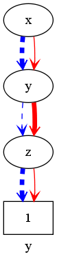
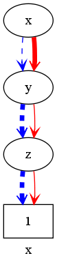
This site will visually introduce polynomial representations as ZDD. A Boolean polynomial is a (multivariate) polynomial over the finite field with two elements, where every exponent is at most one per variable Using ZDDs we describe a term structure of a Boolean polynomial. A term occurs in it, if a valid path (ending at one) corresponds to it: a variable occurring in the polynomial, if and only if the path follows a then branch in the graph.We start with a variable x:
Multiplication
Example: x
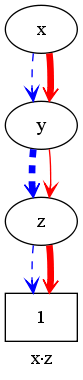
 Multiplying by y we get the image for x*y.
Example: x*y
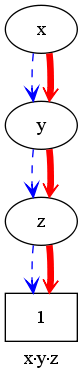
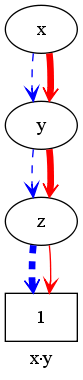
 Analogously we achieve a representation for x*y*z.
Example: x*y*z
 In this way, we see that a monomial looks like a single path trough all its variables leading to the 1 terminal node:
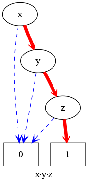
Addition
After getting a picture, how multiplication of variables look like, we have a look at addition:
We the polynomial x+y
Example: x+y
 As we can see, there are now two path leading two the terminal 1-node.


Example: x+y+z
 This of course has three paths leading to the terminal 1-node.


More polynomials
After getting a fundamental understanding for these, very simple polynomials, we try to understand more complicated examples. We add 1 to the polynomial the above presented polynomial x*y*z and get the following picture for x*y*z+1:Example: x*y*z+1
 As we can see, we have instead all else-edges pointing to zero a valid path pointing to one by choosing the else branch from the root polynomial, which yields in some sense the empty path corresponding to the term 1.


Example: x*y*z+x
 As we can see, this else edge leading to the terminal one-node moves down, as this term now starts with x.


Example: x*y*z+y
 In the first moment the graph might look surprisingly different. In reality the path describing the second summand, just changes the order of it's branches:
First we take the else branch at the node representing the variable x (as the term y doesn't contain x), then the then branch at y.
In the image above, we had just the opposite order of branches.
In the first moment the graph might look surprisingly different. In reality the path describing the second summand, just changes the order of it's branches:
First we take the else branch at the node representing the variable x (as the term y doesn't contain x), then the then branch at y.
In the image above, we had just the opposite order of branches.


Example: x*y*z+z
 In comparison to the previous example, the left y-node is replaced by a z-node, which is merged with the z-node in the right part of the previous graph


Special sets
In this section, I will represent a few very structured polynomials with a structured diagram. First of all, I represent the polynomial (a+1)*(b+1)*(c+1)*(d+1)*(e+1) containing every monomial in the variables a, b, c, d, e. The polynomials has 32 terms, but the graph contains only 5 non-terminal nodes and 10 edges. Starting from the root node, on each of the five levels, we can choose the then or else branch and will always end at the terminal 1-node (so get a valid path). Combinatorial this means, that we have five times a choices of two possibilities, so we get 32 combinations, which is exactly the number of terms.Example: (a+1)*(b+1)*(c+1)*(d+1)*(e+1)
*(b+1)*(c+1)*(d+1)*(e+1)") In the following, we restrict the degree for each terms to a maximum of two to represent the polynomial: a*(b+c+d+e)+b*(c+d+e)+c*(d+e)+d*e+a+b+c+d+e+1
In the following, we restrict the degree for each terms to a maximum of two to represent the polynomial: a*(b+c+d+e)+b*(c+d+e)+c*(d+e)+d*e+a+b+c+d+e+1
Example: a*(b+c+d+e)+b*(c+d+e)+c*(d+e)+d*e+a+b+c+d+e+1
+b*(c+d+e)+c*(d+e)+d*e+a+b+c+d+e+1") Again, following the diagram, every path leads to the 1-node, so is valid.
On the other hand, it is not possible to take more than two times a then-branch, as at the latest after the second then branch the path reaches the terminal node.
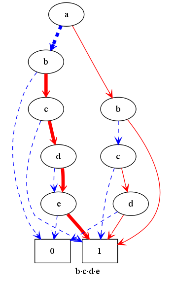
The next variation of the polynomial will only contain of exactly degree two: a*(b+c+d+e)+b*(c+d+e)+c*(d+e)+d*e
The difference of the graphs is quite subtle. Two edges lead now to the 0-node, which means that the path is not valid and the corresponding term does not occur in the polynomial. It is obvious to see, that this makes exactly end those path at 0, which take only zero or one then branch, so have the corresponding term has degree strictly smaller than two.
Again, following the diagram, every path leads to the 1-node, so is valid.
On the other hand, it is not possible to take more than two times a then-branch, as at the latest after the second then branch the path reaches the terminal node.
The next variation of the polynomial will only contain of exactly degree two: a*(b+c+d+e)+b*(c+d+e)+c*(d+e)+d*e
The difference of the graphs is quite subtle. Two edges lead now to the 0-node, which means that the path is not valid and the corresponding term does not occur in the polynomial. It is obvious to see, that this makes exactly end those path at 0, which take only zero or one then branch, so have the corresponding term has degree strictly smaller than two.
Example: a*(b+c+d+e)+b*(c+d+e)+c*(d+e)+d*e
+b*(c+d+e)+c*(d+e)+d*e")
Lexicographical ordering/Natural path ordering
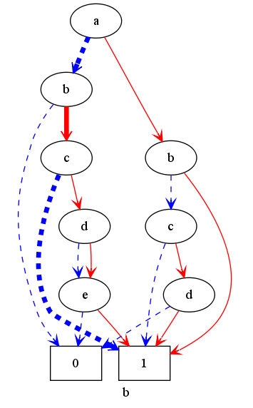
In all these examples, the rightmost path consists only of then branches and leads to the terminal 1-node. While the first is of course a consequence of, that we try to let then branches go to the right, the second might be in the first moment surprising, but is very general and reflects the fact, that ZDDs are reduced (letting out redundant nodes): If the then branch of a node leads to zero, this means that only the else branch (terms in which the variable corresponding to the node doesn't occur) contributes the the term structure of that (sub-) polynomial, so the node doesn't give more information on our term structure and we can leave it out. Note, that other forms of diagrams like ROBDDs can have other rules for the implicit elimination of nodes and its meaning. In this way, always choosing the then path determines a naturally biggest path. This corresponds to searching a term with early variables have an as exponent as high as possible (one), which is the lexicographically leading term of a polynomial. In a similar way we can define a natural order on the valid paths of the graph, which corresponds just to the lexicographical ordering of terms in a Boolean polynomial. The following sequence of images illustrates the natural path ordering. Each picture highlights an path (ordered by the natural ordering, which corresponds to the lexicographical monomial ordering).


We provide a second less structured example, which shows the natural ordering of path: the polynomial a*b + a*c*d + a + b*c*d*e + b*c*e + b


This explains, why the lexicographical ordering works very natural for polynomials in ZDD representation. However, we have implemented quite sophisticated implementations of important other orderings (leading term calculation and ordered iteration) in PolyBoRi:
- Degree lexicographical ordering
- (Ascending) Degree reverse lexigraphical ordering
- Block orderings (for degree ordered blocks)
To contrast the natural path ordering, we display the paths of the same polynomial now in degree lexicographical ordering.


Also for the second example (a*b + a*c*d + a + b*c*d*e + b*c*e + b), we show the ordering of paths corresponding to degree lexicographical ordering


The iterators implemented in PolyBoRi calculate successively the valid paths of a ZDD (terms of the polynomial). This calculation of the next path depends essentially just on the current path. Moreover they use only the ZDD structure of the polynomial, to avoid conversions. This is very important for performance, if you iterate just over the first few terms.
Dependence of ZDDs on the order of variables
It is quite obvious, that the form of the ZDDs depends on the ordering of variables: In the trivial cases, just some nodes are switch. However, usually the ZDD can look very different.
We start with an easy example: The polynomial a*b+a*c+a+1
Example: a*b+a*c+a+1

If we reverse the ordering of variables, the image just looks as follows:
Example: a*b+a*c+a+1, reversed order
 We continue with a slightly more complex example: The polynomial a*b*c+a*b+a*c+1
Example: a*b+a*c+a+1

Again, the reversing the ordering of variables, changes the form of the ZDD:
Example: a*b+a*c+a+1, reversed order

While the differences above were in an expectable magnitude and the polynomials looked quite artificial, we continue with the highest carry BIT of an 3-bit adder. First we start we the naive alphabetical ordering of variables:
Example: Carry BIT 3-bit adder

The ZDD looks quite huge and not very structured. But if we optimize the ordering of variables, the graph looks like that:
Example: Carry BIT 3-bit adder, topological ordered

Using this ordering of variables makes also the polynomial computations much faster.
